Isaac Sim Speedup Cheat Sheet

The speed of the simulation is primarily determined by the physics step size and the minimum simulation frame rate. However, these settings can be influenced by other factors such as the complexity of the scene, the number of physics objects, and the computational resources available.

Here are some suggestions to speed up your simulation:

1. Physics Step Size: The physics step size determines the time interval for each physics simulation step. A smaller step size will result in a more accurate simulation but will also require more computational resources and thus slow down the simulation. Conversely, a larger step size will speed up the simulation but may result in less accurate physics. You can adjust the physics step size in your script using the world.set_physics_step_size(step_size) function, where step_size is the desired step size in seconds.

2. Minimum Simulation Frame Rate: The minimum simulation frame rate determines the minimum number of physics simulation steps per second. If the actual frame rate drops below this value, the simulation will slow down to maintain the accuracy of the physics. You can adjust the minimum simulation frame rate in your script using the world.set_min_simulation_frame_rate(frame_rate) function, where frame_rate is the desired frame rate in frames per second.

3. GPU Dynamics: Enabling GPU dynamics can potentially speed up the simulation by offloading the physics calculations to the GPU. However, this will only be beneficial if your GPU is powerful enough and not already fully utilized by other tasks. If enabling GPU dynamics slows down the simulation, it may be that your GPU is not able to handle the additional load. You can enable or disable GPU dynamics in your script using the world.set_gpu_dynamics_enabled(enabled) function, where enabled is a boolean value indicating whether GPU dynamics should be enabled.

4. Optimize the Scene: As mentioned in the previous response, optimizing the scene can also help to speed up the simulation. This includes reducing the complexity of the scene, implementing level of detail (LOD), culling invisible objects, and optimizing the physics settings.

5. Manually Set Thread Count: overwriting the omni.physx GPU setting and increasing the thread count

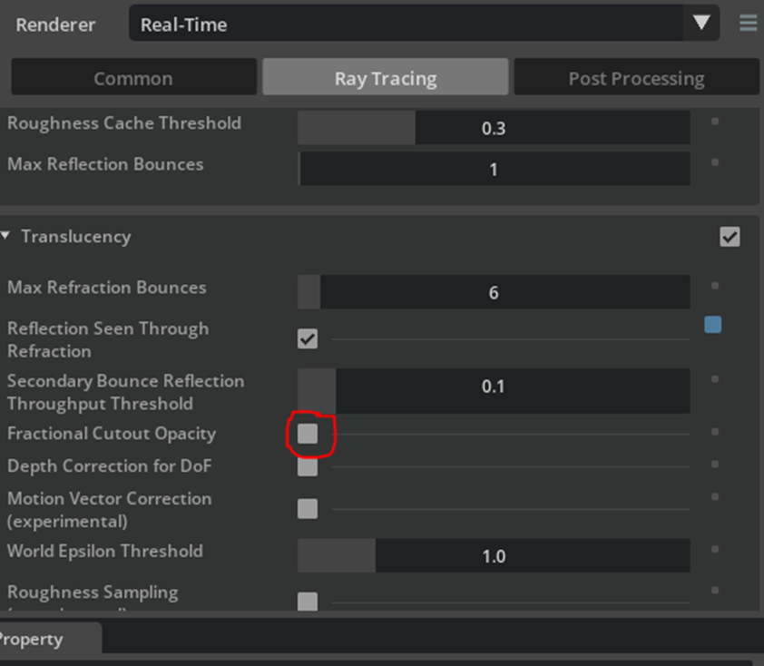
6. Verify using RTX – Realtime Mode: (see here) Note that this affects opacity, and user may need to set partial opacity checkbox

7. Disable Materials and Lights: To get simpler/faster rendering you can:

• disabling all materials, set it to -1 to go back to regular.

  import carb
  carb.settings.get_settings().set_int("/rtx/debugMaterialType", 0)
  

• hide lights

• turn off rendering features in the render settings panel (these will also have equivalent carb settings that can be set in python). There is no non-rtx rendering mode in the isaac sim GUI application, but you can disable almost everything (reflections, transparency, etc) to increase execution speed. To disable rendering completely unless explicitly needed by a sensor, you can use the headless application workflow.

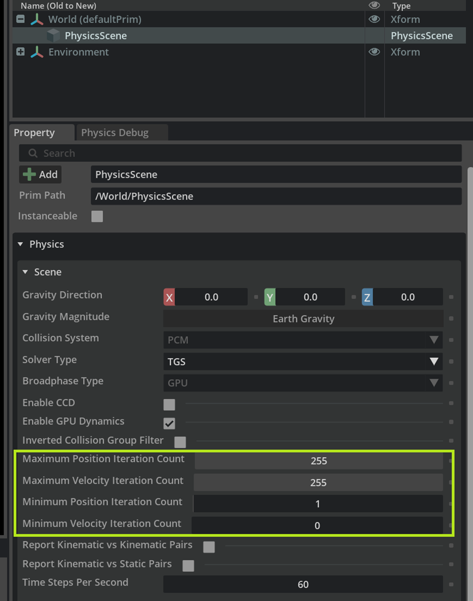
8. OV Solver Settings: Lowering solver iterations to a count that still results in acceptable simulation fidelity will help a lot with performance. You can set global iteration clamps in the scene.

9. CPU and GPU Simulation Depending on Scene Size: there is a minimum floor to the cost of using the GPU. For the smallest simulations, there may not be a benefit to the I/O transfer costs, and relying simply on the CPU may be optimal. If you are simulating only a few rigid bodies and articulations, it is likely beneficial to switch to CPU simulation. If you are simulating large scenes, for example in an RL setting, you should use the GPU simulation and access simulation state using a batch API, e.g. an articulation view.

10. Render Transforms in Runtime Fabric: It is expensive to write back render transforms and other simulation state to USD and you should use the physics Fabric extension instead (see PhysX for details about Fabric).

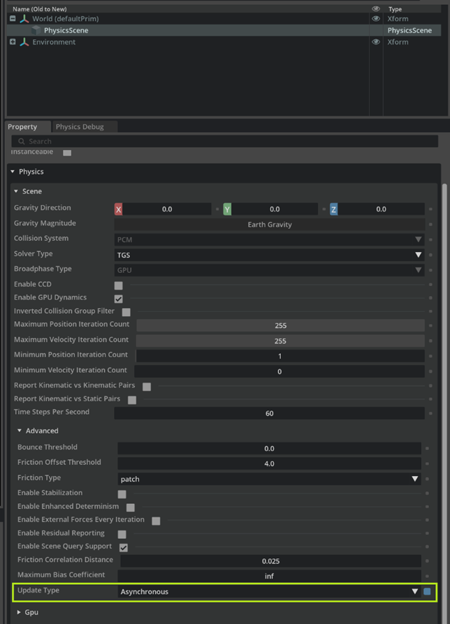
11. Asynchronous Simulation and Rendering: In the scene settings, you can try the async update setting to run simulation and rendering in parallel. This is ideal for simulations that do not need to run custom Python code every step, since Python can have issues when it is called from a separate thread.

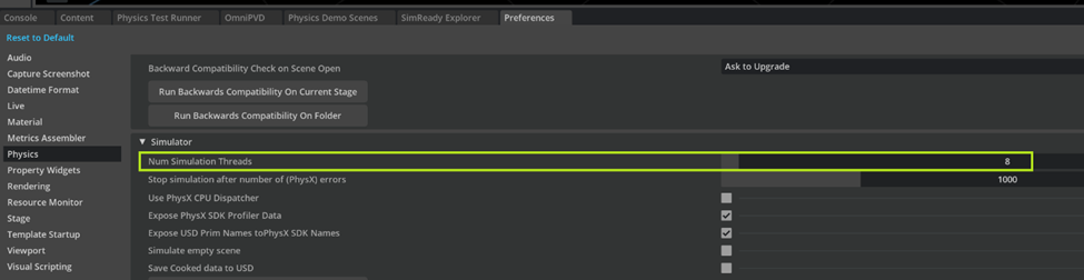
12. Physics Thread Count: You may adjust the number of CPU threads used for simulation. We have seen cases where lower thread counts result in a speedup. This can be changed in the Preferences tab, Physics section. Using 0 here runs the simulation single-threaded, which usually gives the best performance for small scenes.

13. Unintended Collision Geometry Overlap: When setting up reinforcement learning simulation scenes with many parallel environments, make sure that you do not duplicate collision geometry such as ground planes that will generate a lot of inter-environment overlaps that are expensive to check in the collision phase. Below is an example of an incorrectly setup scene, where the ground plane in the environment has been duplicated many times. Since a ground plane is infinite, each one touches all the environments, leading to performance and memory usage problems.

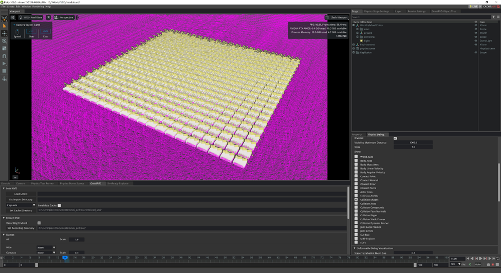
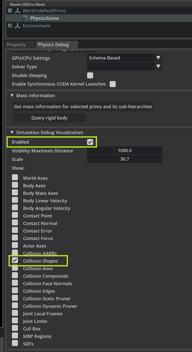
Use the PhysX debug visualization (as enabled in the screenshot below) to inspect the scene and visually confirm that everything looks fine. In the above screenshot, the visual hint that something is wrong is the unexpected sea of magenta debug lines all around the scene.

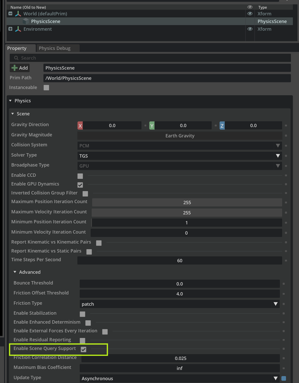
14. Disable Scene Query Support: If you are not using scene queries, you may disable support for it to improve performance. This can be changed in the Property panel of a PhysicsScene.

15. Multi-GPU Render and Simulation: If your machine has multiple GPUs, setup the simulation and render to use two distinct GPUs.

16. Collision Geometry Choice: The simpler the collision geometry, the faster the simulation. For example, an SDF mesh collider will be more expensive than a simple sphere.

17. Deformable or Particle Features: Deformables and particles are considerably more expensive to simulate than rigid bodies. Instead of deformables, you may want to experiment with rigid bodies and compliant contacts, or rigid bodies connected with joints to approximate a deformable geometry.

18. Python Callbacks: Users can implement per-physics-step or simulation-event callbacks in Python. It is good to be aware that this callback code can become a bottleneck.

19. Update drivers and software

Checkout the Physics Simulation Performance guide for more optimization tricks!